Chapter 6 Model training
Model training in supervised ML is guided by the match (or mismatch) between the predicted and observed target variable(s), that is, between \(\hat{Y}\) and \(Y\). The loss function quantifies this mismatch (\(L(\hat{Y}, Y)\)), and the algorithm takes care of progressively reducing the loss during model training. Let’s say the ML model contains two parameters and predictions can be considered a function of the two (\(\hat{Y}(w_1, w_2)\)). \(Y\) is actually constant. Thus, the loss function is effectively a function \(L(w_1, w_2)\). Therefore, we can consider the model training as a search of the parameter space of the machine learning model \((w_1, w_2)\) to find the minimum of the loss. Common loss functions are the root mean square error (RMSE), or the mean square error (MSE), or the mean absolute error (MAE). Loss minimization is a general feature of ML model training.
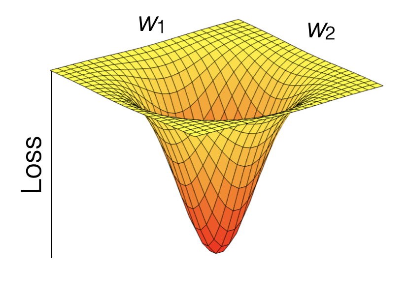
Figure 6.1: Visualization of a loss function as a plane spanned by the two parameters \(w_1\) and \(w_2\).
Model training is implemented in R for different algorithms in different packages. Some algorithms are even implemented by multiple packages (e.g., nnet and neuralnet for artificial neural networks). As described in Chapter 4, the caret package provides “wrappers” that handle a large selection of different ML model implementations in different packages with a unified interface (see here for an overview of available models). The caret function train() is the centre piece. Its argument metric specifies the loss function and defaults to the RMSE for regression models and accuracy for classification (see sub-section on metrics below).
6.1 Hyperparameter tuning
Practically all ML algorithms have some “knobs” to turn in order to achieve efficient model training and predictive performance. Such “knobs” are the hyperparameters. What these knobs are, depends on the ML algorithm.
For KNN, this is k - the number of neighbours to consider for determining distances. There is always an optimum \(k\). Obviously, if \(k = n\), we consider all observations as neighbours and each prediction is simply the mean of all observed target values \(Y\), irrespective of the predictor values. This cannot be optimal and such a model is likely underfit. On the other extreme, with \(k = 1\), the model will be strongly affected by the noise in the single nearest neighbour and its generalisability will suffer. This should be reflected in a poor performance on the validation data.
For random forests from the ranger package, hyperparameters are:
mtry: the number of variables to consider to make decisions, often taken as \(p/3\), where \(p\) is the number of predictors.min.node.size: the number of data points at the “bottom” of each decision treesplitrule: the function applied to data in each branch of a tree, used for determining the goodness of a decision
Hyperparameters usually have to be “tuned”. The optimal setting depends on the data and can therefore not be known a priori.
In caret, hyperparameter tuning is implemented as part of the train() function. Values of hyperparameters to consider are to be specified by the argument tuneGrid, which takes a data frame with column(s) named according to the name(s) of the hyperparameter(s) and rows for each combination of hyperparameters to consider.
## do not run
train(
  form = GPP_NT_VUT_REF ~ SW_F_IN + VPD_F + TA_F,
  data = ddf,
  method = "ranger",
  tuneGrid = expand.grid( .mtry = floor(6 / 3),
                          .min.node.size = c(3, 5, 9,15, 30),
                          .splitrule = c("variance", "maxstat")),
  ...
)
Here, expand.grid() is used to provide a data frame with all combinations of values provided by individual vectors.
6.2 Resampling
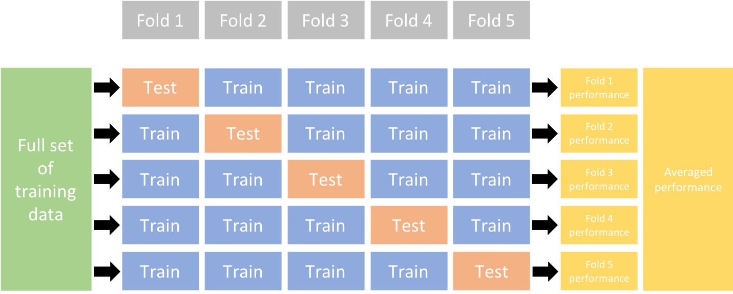
The goal of model training is to achieve the best possible model generalisability. That is, the best possible model performance when predicting to data that was not used for training - the test data. Resampling mimicks the comparison of predictions to the test data. Instead of using all training data, the training data is resampled into a number further splits into pairs of training and validation data. Model training is then guided by minimising the average loss determined on each resample of the validation data. Having multiple resamples (multiple folds of training-validation splits) avoids the loss minimization from being misguided by random peculiarities in the training and/or validation data.
A common resampling method is k-fold cross validation, where the training data is split into k equally sized subsets (folds). Then, there will be k iterations, where each fold is used for validation once (while the remaining folds are used for training). An extreme case is leave-one-out cross validation, where k corresponds to the number of data points.
To do a k-fold cross validation during model training in R, we don’t have to implement the loops around folds ourselves. The resampling procedure can be specified in the caret function train() with the argument trControl. The object that this argument takes is the output of a function call to trainControl(). This can be implemented in two steps. For example, to do a 10-fold cross-validation, we can write:
## do not run
train(
  pp,
  data = ddf_train,
  method = "ranger",
  tuneGrid = expand.grid( .mtry = floor(6 / 3),
                          .min.node.size = c(3, 5, 9,15, 30),
                          .splitrule = c("variance", "maxstat")),
  trControl = trainControl(method = "cv", number = 10),
  ...
)
In certain cases, data points stem from different “groups”, and generalisability across groups is critical. In such cases, data from a given group must not be used both in the training and validation sets. Instead, splits should be made along group delineations. The caret function groupKFold() offers the solution for this case.