Chapter 2 Introduction
2.1 Learning objectives
In this workshop, we use ecosystm flux data and parallel measurements of meteorological variables to model ecosystem gross primary production (the ecosystem-level CO2 uptake by photosynthesis). These data and prediction task is used to introduce fundamental methods of machine learning (data splitting, model training, random forest algorithm) and their implementations in R. After this course, you will …
- Understand how overfitting models can happen and how it can be avoided.
- Implement a typical workflow using a machine learning model for a supervised regression problem.
- Evaluate the power of the model.
- Visualise results.
2.2 Some primers
Machine learning (ML) refers to a class of algorithms that generate statistical models of data. There are two main types of machine learning:
Unsupervised machine learning: Detecting patterns without prior specification.
Supervised machine learning: Model fitting by optimising predictions for a given target.
Loss is a function predicted and observed values derived from the validation set. It is minimised during model training.
2.3 Overfitting
This example is based on this example from scikit-learn.
Machine learning (ML) may appear magical. The ability of ML algorithms to detect patterns and make predictions is fascinating. However, several challenges have to be met in the process of formulating, training, and evaluating the models. In this practical we will discuss some basics of supervised ML and how to achieve best predictive results.
In general, the aim of supervised ML is to find a model \(\hat{Y} = f(X)\) that is trained (calibrated) using observed relationships between a set of features (also known as predictors, or labels, or independent variables) \(X\) and the target variable \(Y\). Note, that \(Y\) is observed. The hat on \(\hat{Y}\) denotes an estimate. Some algorithms can even handle predictions of multiple target variables simultaneously (e.g., neural networks). ML algorithms consist of (more or less) flexible mathematical models with a certain structure and set of parameters. At the simple extreme end of the model spectrum is the univariate linear regression. You may not want to call this a ML algorithm because there is no iterative learning involved. Nevertheless, also univariate linear regression provides a prediction \(\hat{Y} = f(X)\), just like other (proper) ML algorithms do. The functional form of a linear regression is not particularly flexible (just a straight line for the best fit between predictors and targets) and it has only two parameters (slope and intercept). At the other extreme end are, for example, deep neural networks. They are extremely flexible, can learn highly non-linear relationships and deal with interactions between a large number of predictors. They also contain very large numbers of parameters, typically on the order of thousands. You can imagine that this allows these types of algorithms to very effectively learn from the data, but also bears the risk of overfitting.
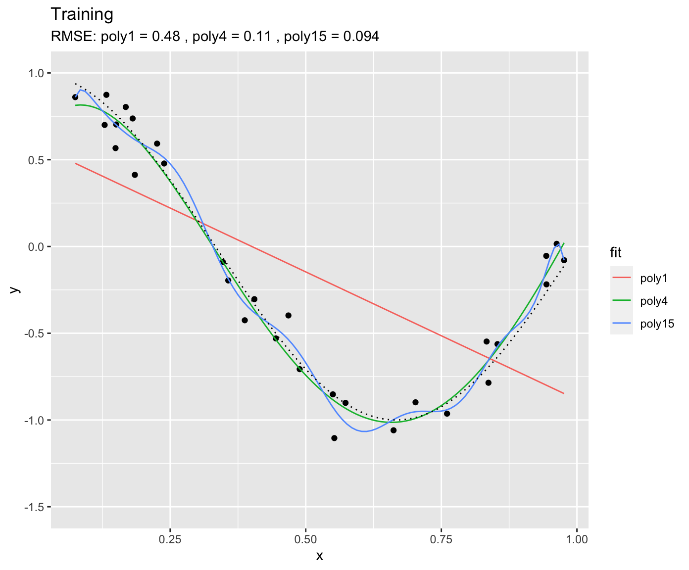
What is overfitting? The following example illustrates it. Let’s assume that there is some true underlying relationship between a predictor \(x\) and the target variable \(y\). We don’t know this relationship (in the code below, this is true_fun()) and the observations contain a (normally distributed) error (y = true_fun(x) + 0.1 * rnorm(n_samples)). Based on our training data (df_train), we fit three polynomial models of degree 1, 4, and 15 to the observations. A polynomial of degree N is given by: \[
y = \sum_{n=0}^N a_n x^n
\] \(a_n\) are the coefficients, i.e., model parameters. The goal of the training is to get the coefficients \(a_n\). From the above definition, the polynomial of degree 15 has 16 parameters, while the polynomial of degree 1 has two parameters (and corresponds to a simple linear regression). You can imagine that the polynomial of degree 15 is much more flexible and should thus yield the closest fit to the training data. This is indeed the case.
We can use the same fitted models on unseen data - the validation data. This is what’s done below. Again, the same true underlying relationship is used, but we sample a new set of data points in x and add a new sample of errors on top of the true relationship.
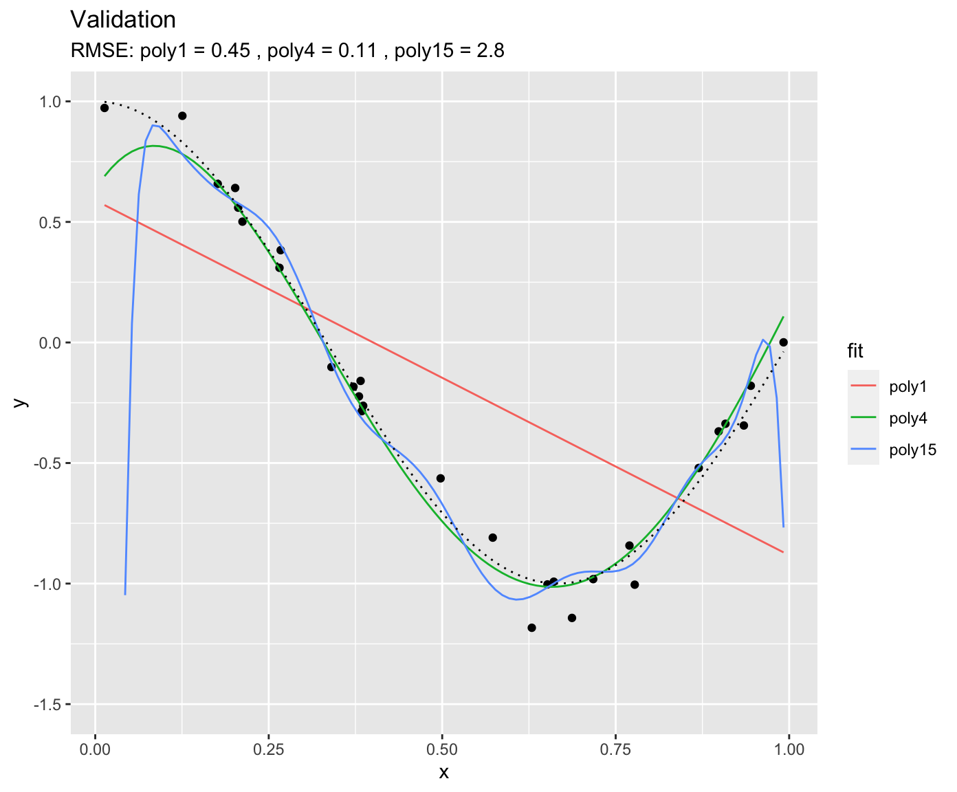
You see that, using the validation set, we find that “poly4” actually performs the best - it has a much lower RMSE that “poly15”. Apparently, “poly15” was overfitted. Apparently, it indeed used its flexibility to fit not only the shape of the true underlying relationship, but also the observation errors on top of it. This has obviously the implication that, when this model is used to make predictions for data that was not used for training (calibration), it will yield misguided predictions that are affected by the errors in the training set. In the above pictures we can also conclude that “poly1” was underfitted.
It gets even worse when applying the fitted polynomial models to data that extends beyond the range in \(x\) that was used for model training. Here, we’re extending just 20% to the right.
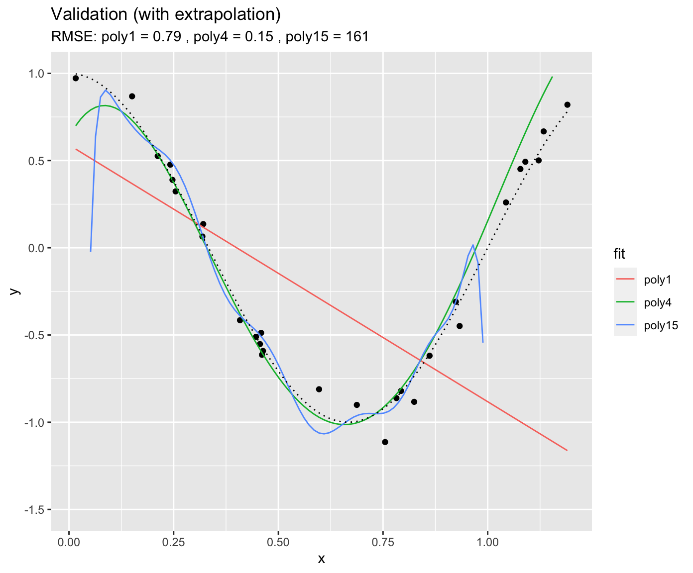
You see that the RMSE for “poly15” literally explodes. The model is hopelessly overfitted and completely useless for prediction, although it looked like it fit the data best when we considered at the training results. This is a fundamental challenge in ML - finding the model with the best generalisability. That is, a model that not only fits the training data well, but also performs well on unseen data.
The phenomenon of fitting/overfitting as a function of the model “flexibility” is also referred to as bias vs. variance trade-off. The bias describes how well a model matches the training set (average error). A model with low bias will match the data set closely and vice versa. The variance describes how much a model changes when you train it using different portions of your data set. “poly15” has a high variance, but much of its variance is the result of misled training on observation errors. On the other extreme, “poly1” has a high bias. It’s not affected by the noise in observations, but its predictions are also far off the observations. In ML, we are challenged to balance this trade-off. In Figure ?? you can see a schematic illustration of the bias–variance trade-off.
This chapter introduces the methods to achieve the best model generalisability and find the sweet spot between high bias and high variance. The steps to get there include the preprocessing of data, splitting the data into training and testing sets, and model training that “steers” the model towards what is considered a good model fit in terms of its generalisation power.
You have learned in video 6a about the basic setup of supervised ML, with input data containing the features (or predictors) \(X\), predicted (\(\hat{Y}\)) and observed target values (\(Y\), also known as labels). In video 6b (title 6c: loss and it’s minimization), you learned about the loss function which quantifies the agreement between \(Y\) and \(\hat{Y}\) and defines the objective of the model training. Here, you’ll learn how all of this can be implemented in R. Depending on your application or research question, it may also be of interest to evaluate the relationships embodied in \(f(X)\) or to quantify the importance of different predictors in our model. This is referred to as model interpretation and is introduced in the respectively named subsection. Finally, we’ll get into feature selection in the next Application session.
The topic of supervised machine learning methods covers enough material to fill two sessions. Therefore, we split this part in two. Model training, implementing the an entire modelling workflow, model evaluation and interpretation will be covered in the next session’s tutorial (Supervised Machine Learning Methods II).
Of course, a plethora of algorithms exist that do the job of \(Y = f(X)\). Each of them has its own strengths and limitations. It is beyond the scope of this course to introduce a larger number of ML algorithms. Subsequent sessions will focus primarily on Artificial Neural Networks (ANN) - a type of ML algorithm that has gained popularity for its capacity to efficiently learn patterns in large data sets. For illustration purposes in this and the next chapter, we will briefly introduce two simple alternative “ML” methods, linear regression and K-nearest-neighbors. They have quite different characteristics and are therefore great for illustration purposes in this chapter.
2.4 Our modelling challenge
The environment determines ecosystem-atmosphere exchange fluxes of water vapour and CO2. Temporally changing mass exchange fluxes can be continuously measured with the eddy covariance technique, while abiotic variables (meteorological variables, soil moisture) can be measured in parallel. This offers an opportunity for building models that predict mass exchange fluxes from the environment.
In this workshop, we formulate a model for predicting ecosystem gross primary production (photosynthesis) from environmental covariates.
This is to say that GPP_NT_VUT_REF is the target variable, and other available variables available in the dataset can be used as predictors.
2.5 Data
Data is provided here at daily resolution for a site (‘CH-Dav’) located in the Swiss alps (Davos). This is one of the longest-running eddy covariance sites globally and measures fluxes in a evergreen coniferous forest with cold winters and temperate and relatively moist summers.
For more information of the variables in the dataset, see FLUXNET 2015 website, and Pastorello et al., 2020 for a comprehensive documentation of variable definitions and methods.
2.5.1 Available variables
TIMESTAMP: Day of measurement.TA_F: Air temperature. The meaning of suffix_Fis described in Pastorello et al., 2020.SW_IN_F: Shortwave incoming radiationLW_IN_F: Longwave incoming radiationVPD_F: Vapour pressure deficit (relates to the humidity of the air)PA_F: Atmospheric pressureP_F: PrecipitationWS_F: Wind speedGPP_NT_VUT_REF: Gross primary production - the target variableNEE_VUT_REF_QC: Quality control information forGPP_NT_VUT_REF. Specifies the fraction of high-quality underlying high-frequency data from which the daily data is derived. 0.8 = 80% underlying high-quality data, remaining 20% of the high-frequency data is gap-filled.
2.6 More primers
2.6.1 K-nearest neighbours
As the name suggests, the K-nearest neighbour (KNN) uses the \(k\) observations that are “nearest” to the new record for which we want to make a prediction. It then calculates their average (in regression) or most frequent value (in classification) as the prediction. “Nearest” is determined by some distance metric evaluated based on the values of the predictors. In our example (GPP_NT_VUT_REF ~ .), KNN would determine the \(k\) days where conditions, given by our set of predictors, were most similar (nearest) to the day for which we seek a prediction. Then, it calculates the prediction as the average (mean) GPP value of these days. Determining “nearest” neighbors is commonly based on either the Euclidean or Manhattan distances between two data points \(x_a\) and \(x_b\), considering all \(p\) predictors \(j\).
Euclidean distance: \[ \sqrt{ \sum_{j=1}^p (x_{a,j} - x_{b,j})^2 } \\ \] Manhattan distance: \[ \sum_{j=1}^p | x_{a,j} - x_{b,j} | \]
In two-dimensional space, the Euclidean distance measures the length of a straight line between two points (remember Pythagoras!). The Manhattan distance is called this way because it measures the distance you would have to walk to get from point \(a\) to point \(b\) in Manhattan, New York, where you cannot cut corners but have to follow a rectangular grid of streets. \(|x|\) is the positive value of \(x\) ( \(|-x| = x\)).
KNN is a simple algorithm that uses knowledge of the “local” data structure for prediction. A drawback is that the model training has to be done for each prediction step and the computation time of the training increases with \(x \times p\). KNNs are used, for example, to impute values (fill missing values) and have the advantage that predicted values are always within the range of observed values of the target variable.
2.6.2 Random Forest
Random forest models are based on decision trees, where binary decisions for predicting the target’s values are based on thresholds of the predictors’ values. The depth of a decision tree refers to the number of such decisions. The deeper a tree, the more likely the model will overfit. Here are some links for more information on decision trees:
Just as forests are made up by trees, random Forest models make use of random subsets of the original data and of available predictions and respective decision trees. Predictions are then made by averaging predictions of individual base learners (the decision trees). The number of predictors considered at each decision step is a tunable parameter (a hyperparameter, typically called \(m_{try}\)). Introducing this randomness is effective because decision trees tend to overfit and because of the wisdom of the crowd - i.e., the power of aggregating individual predictions with their random error (and without systematic bias) for generating accurate and relatively precise predictions.
Random forest models have gained particular popularity and are widely applied in environmental sciences not only for their power, but also for their ease of use. No preprocessing (centering, scaling) is necessary, they can deal with skewed data, and can effectively learn interactions between predictors.
Here are some links for more information on random forest: