3  The global carbon budget

The principles of what drives the carbon cycle, and along with it the energy and mass flow, cannot be better explained than through the words of the late and great Richard Feynman - Nobel Prize laureate in Physics and a gifted teacher.

Energy from solar radiation is absorbed and consumed to convert atmospheric C, present in its (oxidized) gaseous form CO₂, into C in carbohydrates and biomass. In other words, biomass stores solar energy. This energy can be released again, not only through combustion (fire). It also serves as an energy source through consumption of organic matter by heterotrophic organisms - animals (including humans), fungi, and bacteria. Fire and heterotrophic consumption release CO₂ and thus close the atmosphere-land C cycle.

The fact that the mass of trees comes from the air, not from the soil was discovered in the late 1600 by Jan Baptista van Helmont, a Belgian chemist, physiologist, and physician. Van Helmont conducted an experiment to understand the source of plant growth. He planted a willow tree in a pot with a measured amount of soil and watered it with only rainwater. After five years, he found that the tree had gained a significant amount of biomass, while the soil weight had barely changed. Mass conservation appeared to have been violated. Has it?

Van Helmont concluded that the increase in plant mass did not come from the soil, as he initially believed, but rather from the water. Apparently, he didn’t fully grasp the role of photosynthesis for fixing gaseous carbon dioxide (CO₂) from the air. The respective C is partly converted to wood, leaves, and roots, and makes up around 50% of a tree’s biomass. Anyways, his experiment laid the groundwork for later discoveries about the vital role of CO₂ in plant growth. The understanding of photosynthesis and the role of CO₂ in plant carbon uptake was further developed later and will be introduced in Chapter 4.

The C cycling between the atmosphere and the ocean mostly follows very different processes and dynamics than the carbon uptake and release on land. These processes and implications for CO₂ trajectories are introduced in Chapter 13. The global pools of the land, ocean, and atmosphere C and the fluxes between them, and how they are changing as a result of anthropogenic fossil fuel combustion, is the topic of this chapter.

3.1 The pre-industrial carbon cycle

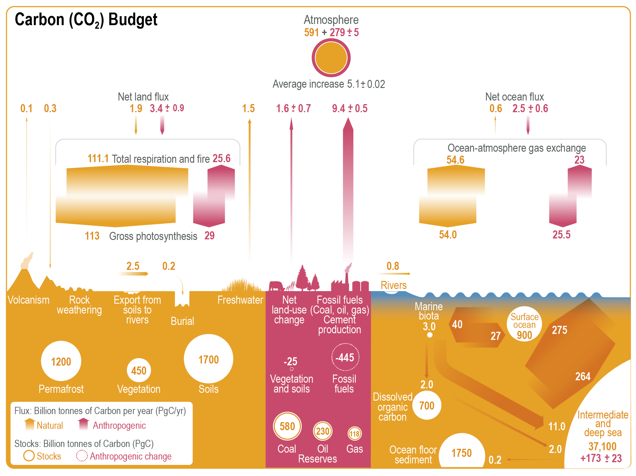
Carbon is an abundant element, present in all organic matter - matter produced by biota (living organisms) - and in inorganic forms in the atmosphere, the ocean, and the lithosphere. On land, the vast majority of C is present in organic forms in living biomass - mostly of vegetation (450 PgC) and soil organic matter (1700 PgC excluding permafrost). Of the latter, a particularly large stock of C is stored in permafrost soils (1200 PgC). In the ocean, the vast majority of C mass is present in inorganic forms, dissolved in ocean water, of which 900 PgC is stored in the surface ocean (the well-mixed top few hundred meters) and 37,100 PgC is stored in the deep ocean. Dissolved organic carbon in the ocean makes up 700 PgC and 1750 PgC are stored as carbonate shells in ocean floor sediments. In the pre-industrial Earth, 591 PgC were present as CO₂ in the atmosphere.

Note

We will express all carbon fluxes and pools in units of mass C. For global-scale quantities, we use PgC:

1 PgC = 1 petagram C = 10¹⁵ gC = 10⁹ tC = 1 GtC = 1 gigaton C.

C mass is sometimes also expressed in units of mass CO₂. The interconversion between mass C and mass CO₂ has to consider the respective molecular masses (44.01 g mol^-1 for CO₂ and 12.011 g mol^-1 for C):

3.664 PgCO₂ contains 1 PgC.

Note

The concentration of CO₂ in the atmosphere is measured in parts per million (ppm), expressed as a dry-air mole fraction. Therefore, ppm is an abbreviation for micromoles per mole dry air. Since the total mass of the atmosphere is well-known and CO₂ is relatively well-mixed in the troposphere within one year, the CO₂ concentration can directly be converted into a total atmospheric mass of C in the form of CO₂ (Ballantyne et al. 2012):

1 ppm CO₂ = 2.124 PgC

Figure 3.1: Global carbon (CO₂) budget (2010–2019). Yellow arrows represent annual carbon fluxes (in PgC yr^-1) associated with the natural carbon cycle, estimated for the time prior to the industrial era, around 1750. Pink arrows represent anthropogenic fluxes averaged over the period 2010–2019. The rate of carbon accumulation in the atmosphere is equal to net land-use change emissions, including land management plus fossil fuel emissions, minus land and ocean net sinks (plus a small budget imbalance). Circles with yellow numbers represent pre-industrial carbon stocks in PgC. Circles with pink numbers represent anthropogenic changes to these stocks (cumulative anthropogenic fluxes) since 1750. The relative change of gross photosynthesis since pre-industrial times is based on 15 Dynamic Global Vegetation Models. The corresponding emissions by total respiration and fire are those required to match the net land flux, exclusive of net land-use change emissions which are accounted for separately. The cumulative change of anthropogenic carbon in the terrestrial reservoir is the sum of carbon cumulatively lost by net land-use change emissions, and net carbon accumulated since 1750 in response to environmental drivers (warming, rising CO₂, nitrogen deposition). Figure from Canadell et al. (2021).

Under the relatively stable climate of the pre-industrial Holocene (11,700 yr BP - 1750 CE), the size of the C pools described above remained relatively stable. To simplify, we can conceive them as constant (at steady state) under the pre-industrial Holocene climate. This is a simplification. For example, millennial-scale trends in solar radiation inputs over the seasons and latitudes (driven by slight changes in the Earth’s orbit around the sun), caused climate and vegetation changes that were substantial and in certain cases abrupt (e.g., the demise of the Green Sahara between around 6-3 ka BP (Shanahan et al. 2015)).

Even under such a pre-industrial steady state, C fluxes between the major reservoirs or pools (atmosphere, ocean, land) persisted. This is indicated in Figure 3.1 by the wide orange arrows pointing up and down between the land and the atmosphere and between the ocean and the atmosphere, as well as between different pools within the ocean. In a steady state, the C flux from the atmosphere into the land roughly equals the flux from the land to the atmosphere, and the net exchange flux is zero. Hence, the pool sizes remain constant in spite of the ongoing exchange fluxes between them. We speak of a dynamic equilibrium.

3.2 Carbon pool dynamics

The 1st-order decay model

The concept of pools and fluxes is central for describing and modelling the carbon cycle and other biogeochemical cycles in the environment. The dynamics of a pool $C(t)$ is given by the balance of the flux of C into that pool $I(t)$ and the flux $O(t)$ leaving the pool - over time $t$. In general terms, we can write the temporal change of the pool size as

$$\begin{array}{}\text{(3.1)}& \frac{\mathrm{d}C(t)}{\mathrm{d}t}=I(t)-O(t).\end{array}$$

To simplify the expressions, we will omit $(t)$ below. But remember, that the fluxes and pools vary with time. The assumption that the out-flux $O$ scales linearly with the size of the pool $C$ is a good simplifying description (i.e., a model) for many processes in the environment. For example, the amount of CO₂ produced by the decomposition (decay) of organic matter in the soil scales roughly linearly with the amount of organic matter that is being respired. This leads to the 1st-order decay model of pool dynamics:

$$\begin{array}{}\text{(3.2)}& \frac{\mathrm{d}C}{\mathrm{d}t}=I-kC.\end{array}$$ Here, $k$ is a decay constant and is in units of the inverse of time. In other words, it specifies the fraction of $C$ decaying per unit time (e.g,. seconds, or years). The higher $k$, the more rapidly the pool decays. For the case of $I=0$, we get $\mathrm{d}C/\mathrm{d}t=-kC$. This is a differential equation and can be understood as: What is the function that yields itself, multiplied by $-k$, when taking its derivative with respect to time? The solution is:

$$C(t)=C_0{e}^{-kt}.$$ For example, following this model, the pool of C in soil organic matter would decay exponentially if inputs (litterfall) were zero. The decay constant $k$ determines how long it takes for it to be reduced by a certain factor. A commonly used factor is 0.5. We can calculate a half-life - the time $t$ at which $C(t)=0.5C_0$.

In a dynamic equilibrium the change in the pool size $C$ is by definition zero. $$\begin{array}{}\text{(3.3)}& \frac{\mathrm{d}C}{\mathrm{d}t}=0.\end{array}$$ Combining Equation 3.2 and Equation 3.3 and re-arranging terms leads to the steady-state pool size as a function of the in-flux and the decay constant $k$. $$\begin{array}{}\text{(3.4)}& C^{\ast }=I/k\end{array}$$ Here, the asterisk denotes that $C$ is at steady-state. This solution indicates two aspects. First, the size of the steady-state pool is proportional to the input flux. Note that we assumed that the input flux itself has no dependency on $C$. Second, the size of the steady-state pool is inversely proportional to the decay constant. That is, the faster the decay, the smaller the steady state pool.

Equation 3.2 can also be expressed in terms of an average lifetime or turnover time $\tau$, instead of $k$: $$\begin{array}{}\text{(3.5)}& \frac{\mathrm{d}C}{\mathrm{d}t}=I-C/\tau .\end{array}$$

Exercise

1. Consider the C pool of the intermediate and deep sea (37,100 PgC) in Figure 3.1 (bottom right). What is the turnover time of C in that pool?
2. Express the steady-state pool size $C^{\ast }$ as a function of the in-flux and the turnover time $\tau$.
3. Express the half-life constant as a function of $k$.
4. Do you know about other processes in nature that can be described by the 1st-order decay model?

With the information in Figure 3.1 about pool sizes and steady-state gross fluxes (parallel input and output fluxes), and our model of pool dynamics, we get an insight about how fast C is cycling in and out of different pools. $k=I/C^{\ast }$ is a measure of this cycling rate. Or expressed in terms of its inverse, the turnover time $\tau$ measures how long a C atom resides in that pool. Table 3.1 documents the turnover times for major pools of the global carbon cycle. The small C burial fluxes into sediments on land and on the ocean floor are the supply of what is eventually converted into the very large pool of C in carbonate rock (limestone). A small fraction of the C burial flux is in the form of organic matter, including dead plants, algae, and other microorganisms. Under high heat and pressure, a fraction of it contributes to the formation of hydrocarbons such as oil and gas - fossil fuels. The discrepancy in turnover times between the lithosphere C pool and the other pools indicates that C cycles on vastly different time scales and the slow geological C cycle is largely disconnected from “fast” C cycle between the atmosphere, ocean, and biosphere. Reflecting this discrepancy in time scales, the geological C cycle is not depicted in Figure 3.1 and C in fossil fuel reservoirs is treated as an external input to the fast C cycle.

Table 3.1: Pre-industrial pool sizes, input fluxes, and turnover times of major pools of the global carbon cycle. The preindustrial input flux into the atmosphere is calculated as the sum of fluxes from volcanism, total respiration and fire, freshwater, and ocean-atmosphere gas exchange from Figure 3.1. The input flux into the surface ocean is the sum of ocean-atmosphere gas exchange and the flux from intermediate and deep sea. The flux from marine biota is not additional to the ocean-atmosphere exchange flux. The pool size of the biosphere is taken as the sum of vegetation and soils. The permafrost C pool is relatively inert. The size of the lithosphere C pool includes C in the form of sedimentary (carbonate) rocks and kerogens (solid, insoluble organic matter in sedimentary rocks). Its estimate is based on Falkowski et al. (2000). The input flux into the lithosphere is calculated as the sum of burial on land, rock weathering, and ocean floor sedimentation

Pool	Pool size (PgC)	Input flux (PgC yr-1)	Turnover time (yr)
Atmosphere	591	167.3	3.5
Surface ocean	900	329	2.7
Deep ocean	37,000	(see exercise 3.1)	(see exercise 3.1)
Biosphere	2150	113	19
Lithosphere	75,000,000	0.7	108

It should be noted that the turnover time $\tau$ describes the average time that an atom of C resides in the respective pool. This is a simplification. In the C pool ‘terrestrial biosphere’, not every C atom has the same probability of being oxidized and respired as CO₂. Hence, in reality, $\tau$ is a wide distribution, ranging from seconds to years for non-structural carbon derived from photosynthesis, decades to centuries for C in woody biomass, and to millennia for a small fraction of soil organic matter, especially if the C is protected from oxidation, for example in water-logged soils. The turnover time should therefore be understood as a diagnostic, useful for describing the average systems dynamics in a simplified way, and subsuming multiple processes that operate at different time scales, contributing to different portions of C conversion to CO₂.

The range of turnover times (e.g., within the terrestrial biosphere) arise because C is transferred between multiple pools within the biosphere and the ocean. Going to the next more detailed level of abstraction (model representation), multiple C pools in terrestrial ecosystems can be distinguished (e.g., non-structural C, leaves, roots, wood, litter, soil organic matter, microbes). Some C “cascades” through multiple pools, some is quickly respired back into the atmosphere. The interpretation that $k$ equals the inverse of the turnover time $\tau$, and that the turnover time equals the mean age of all C atoms in that pool, and that the mean transit time (the time it takes between an atom of C entering a pool until it exits that pool again) equals $\tau$ is only valid for certain cases, and not for “C cascades” with fluxes between multiple pools. Requirements are that we’re dealing with a single well-mixed pool, that this pool is at steady-state, that it has been so for an infinitely long time, that $I$ and $k$ are constant over time, and the flux leaving the pool is a linear function of the pool size ($O=kC$) (Sierra et al. 2017). The transit time is the same as residence time - a term used more commonly in hydrology.

3.3 The anthropogenic perturbation

Although fossil fuels are formed by natural processes of the C cycle, their combustion can be regarded as an external input of C into the (modern) global C cycle. This is because the time scale at which the reservoir of fossil fuels is depleted (10² yr) stands in stark contrast to the time scale at which it was formed (10⁸ yr, see turnover time of C in the lithosphere in Table 3.1). The C is added in the form of CO₂ to the atmosphere from where it is taken up by the ocean through diffusion and equilibration of the ocean surface water’s CO₂ partial pressure with the atmosphere’s CO₂ partial pressure, and by the terrestrial biosphere through photosynthesis. It is important to note that CO₂ in the atmosphere does not decay through physical or chemical processes, nor are there C sinks on land or in the ocean that remove C away from the “fast” C cycle - except the burial into sediments (see Figure 3.1 and Table 3.1). However the magnitude of the burial fluxes are dwarfed by the magnitude of C inputs through the combustion of fossil fuels and deforestation. Hence, the present-day C emissions drive an accumulation of the total amount of C cycling in the “fast” C cycle and the added C gets redistributed between the spheres. The net fluxes from the atmosphere into land ecosystems and the ocean arise because the total terrestrial and oceanic C pools are increasing as CO₂ is emitted into the atmosphere and the atmospheric CO₂ concentration is rising. In subsequent chapters (Chapter 4 and Chapter 13), we will learn about the processes driving the CO₂ uptake by land and ocean and the dynamics of the C redistribution in the Earth system. In this chapter, we will look at the global C budget - how much C has been emitted by the combustion of fossil fuels and deforestation and how much of this C has accumulated in the atmosphere and how much has been taken up by the ocean and the terrestrial biosphere?

The global C budget can be defined for globally aggregated fluxes as the balance between emissions from fossil fuels $E_{\mathrm{FF}}$ and land use change $E_{\mathrm{LUC}}$ on the left side of the equation and the redistribution of C among the atmosphere, land and ocean. $G_{\mathrm{atm}}$ is the atmospheric growth rate, $S_{\mathrm{ocean}}$ is the net ocean C uptake (also referred to as the ocean sink) and $S_{\mathrm{land}}$ is the net land C uptake (or land sink). A net flux from the atmosphere into the ocean or into land C storage is positive.

$$\begin{array}{}\text{(3.6)}& E_{\mathrm{FF}}+E_{\mathrm{LUC}}=G_{\mathrm{atm}}+S_{\mathrm{ocean}}+S_{\mathrm{land}}\end{array}$$

This terminology is adopted from the Global Carbon Budget (Friedlingstein et al. 2023) and is expressed as global annual total fluxes. The separation of $E_{\mathrm{LUC}}$ and $S_{\mathrm{land}}$ is not straight-forward, but can be understood in a simplified fashion as spatially separated fluxes, whereby the land sink occurs only on areas that are not affected by land use change (LUC). In reality, LUC affects the land sink which complicates a separation of the two components. This is further resolved in Chapter 10.

The values of the global carbon budget components are given in Figure 3.1 for an average across years 2010-2019, where $S_{\mathrm{ocean}}$ corresponds to the ‘net ocean flux’ and $S_{\mathrm{land}}$ corresponds to the the ‘net land flux’ in Figure 3.1. $E_{\mathrm{LUC}}$ corresponds to ‘net land-use change’. The ‘net’ indicates that $E_{\mathrm{LUC}}$ is the net effect between CO₂ emissions from deforestation and C uptake by re-growing forests and afforestations. Note that the annual atmospheric growth rate is not resolved in Figure 3.1. The most recent update of the global carbon budget from Friedlingstein et al. (2023) is given in Table 3.2 as 10-year averages of annual fluxes for years 2013-2022 and cumulative fluxes for the industrial era - years 1750-2022.

Table 3.2: Global carbon budget (in PgC and PgC yr^-1) from the 2023 update by Friedlingstein et al. (2023)

Component	Cumulative 1750-2022	Annual 2013-2022
$E_{\mathrm{FF}}$	480 $\pm$ 25	9.6 $\pm$ 0.5
$E_{\mathrm{LUC}}$	250 $\pm$ 75	1.3 $\pm$ 0.7
$G_{\mathrm{atm}}$	300 $\pm$ 5	5.2 $\pm$ 0.02
$S_{\mathrm{ocean}}$	190 $\pm$ 40	2.8 $\pm$ 0.4
$S_{\mathrm{land}}$	245 $\pm$ 60	3.3 $\pm$ 0.8

Estimates of each global carbon budget compenent are largely independent from each other and rely on different types of observations, data, and methods. $E_{\mathrm{FF}}$ estimates are based on energy statistics and cement production data. Values reported by Friedlingstein et al. (2023) include the cement carbonation sink. Without that sink, the value of $E_{\mathrm{FF}}$ for 2022 would be about 0.2 PgC yr^-1 higher. $E_{\mathrm{LUC}}$ estimates are based on land-use and land-use change data from national statistics and forest carbon “bookkeeping models”. These models use information about vegetation C stocks, forest C re-growth curves, and the fate of C after deforestation and harvesting (e.g., wood products lifetime). Atmospheric CO₂ concentration, and hence the accumulation of C in the atmosphere, is measured directly and bears the least uncertainty among all carbon budget components. The ocean sink is estimated from global ocean CO₂ uptake models and observation-based products. In Friedlingstein et al. (2023), the land sink is estimated from dynamic global vegetation models.

Advances in observations and modelling in recent years now enable the land and ocean sink to be estimated in a “bottom-up fashion” - using models of land and ocean C uptake. Since every component of the global carbon budget is thereby estimated independently, a budget imbalance term $B_{\mathrm{IM}}$ can be defined. A value of zero indicates that models of the land and ocean C uptake exactly match the (better known) emission terms minus the atmospheric growth rate. $$\begin{array}{}\text{(3.7)}& B_{\mathrm{IM}}=E_{\mathrm{FF}}+E_{\mathrm{LUC}}-(G_{\mathrm{atm}}+S_{\mathrm{ocean}}+S_{\mathrm{land}})\end{array}$$

Today, the global carbon budget is well specified thanks to reliable estimates of its individual components. The budget imbalance is only a fraction of the total emissions. Until recently, “bottom-up” estimates of $S_{\mathrm{land}}$ by land C cycle models were deemed insufficient for providing reliable estimates. Instead, $S_{\mathrm{land}}$ was estimated as the budget residual by neglecting $B_{\mathrm{IM}}$ and rearranging terms in Equation 3.7 to solve for $S_{\mathrm{land}}$. In fact, when the IPCC First Assessment Report was published in 1990, the existence of C sink on land was not known and it was treated as the budget imbalance and referred to as the ‘missing sink’. It was stated that “there are possible processes on land which could account for the missing CO₂ (but it has not been possible to verify them)”.

It was only later that the existence of a terrestrial C sink could be more firmly established and quantified thanks to parallel measurements of the atmospheric O₂ and CO₂ concentrations (Keeling, Piper, and Heimann 1996). (In fact, the ratio O₂/N₂ is measured to avoid the much larger measurement uncertainty in absolute O₂ measurements). The ratios of O₂:CO₂ are known from the stoichiometric molecular formulae for photosynthesis (O₂:CO₂ = 1.1), fossil fuel combustion (O₂:CO₂ = 1.4) and ocean uptake (O₂:CO₂ = 0). An ocean O₂ source from marine organisms has to be factored in. Given the total C emissions from fossil fuel combustion, the net land C balance can thus be calculated and the calculation visualized geometrically (Figure 3.2). Note that net emissions from land use change are not considered and the what is termed the “S_land” in Figure 3.2 is actually the net $(S_{\mathrm{land}}-E_{\mathrm{LUC}})$ in Equation 3.6.

Figure 3.2: Global land and ocean carbon sinks deduced from changes in atmospheric CO₂ and O₂ concentrations. The figure is an updated version of Fig. 2 from Keeling, Piper, and Heimann (1996), taken from a recent update of the atmospheric carbon and oxygen budget by Li et al. (2022). In this figure, what is termed ‘S_land’ corresponds to (S_land - E_LUC) as defined in Equation 3.6.

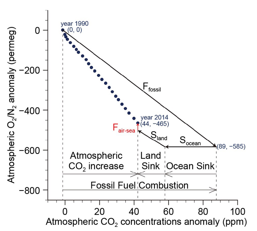
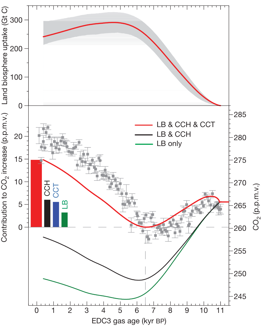
In a mathematical sense, the constraint from atmospheric oxygen can be understood as a second equation, necessary for solving for two unknowns $S_{\mathrm{land}}$ and $S_{\mathrm{ocean}}$. Their sum must equal (well-known) emissions $E_{\mathrm{FF}}+E_{\mathrm{LUC}}$ minus the atmospheric growth rate $G_{\mathrm{atm}}$. This yields only one equation - that for the C budget (Equation 3.6). The oxygen budget provides a second equation and thus enables solving for two unknowns. In a similar fashion, the isotopic composition of C (the ratio of ¹³C:¹²C) also provides a second equation (Joos and Bruno 1998). The history of ¹³C can be measured on ice cores and $(S_{\mathrm{land}}-E_{\mathrm{LUC}})$ can thus be reconstructed for the past (Figure 3.3). Note that in order to separate $S_{\mathrm{land}}$ from the budget, independent estimates of $E_{\mathrm{LUC}}$ are required.

Figure 3.3: Top panel: Cumulative C uptake by the land biosphere over the past 11 kyr. The grey shaded area indicates uncertainty from ice core measurements. Bottom panel: Atmospheric CO₂ concentration (grey squares and modelled atmospheric CO₂ based on scenarios of drivers of past millennial-scale C cycle changes (green: land biosphere is the only driver, black: land biopshere, combined with effects by oceanic carbonate chemistry due to Holocene land C uptake, red: land biosphere, combined with effects by oceanic carbonate chemistry due to Holocene and pre-Holocene land C uptake). Figure from Elsig et al. (2009).

We can adopt the perspective of C cycle science stated in earlier publications. Falkowski et al. (2000) wrote: “Direct determination of changes in terrestrial carbon storage has proven extremely difficult. Rather, the contribution of terrestrial ecosystems to carbon storage is inferred from changes in the concentrations of atmospheric gases, especially CO₂ and O₂ […].” In that sense, let’s consider the land sink to be the budget residual and assume that the ocean sink estimate is accurate (indeed, its uncertainty is only about half the uncertainty in bottom-up land sink estimates, Table 3.2). Visually contrasting emissions and their redistribution reveals an interesting pattern (Figure 3.4). The substantial year-to-year (interannual) variations in the land sink are almost exclusively responsible for interannual variations in the atmospheric growth rate. Total emissions and the ocean sink exhibit little interannual variation. By definition, the sum of the atmospheric growth rate, land and ocean sink is equal to the sum of emissions from fossil fuels and land use change.

Exercise

5. Use Equation 3.7 to express the land sink as the budget residual (assuming $B_{\mathrm{IM}}=0$).

Code

library(readr)
library(here)
library(dplyr)
library(tidyr)
library(ggplot2)

# Data from Friedlingstein et al. 2023. Downloaded excel file 'Global 
# Carbon Budget v2023' from
# https://globalcarbonbudgetdata.org/latest-data.html
# Saved tab Global Carbon Budget as a CSV file. 
# Reading this CSV here.
df <- read_csv(here("data/Global_Carbon_Budget_2023v1.0_tabGlobalCarbonBudget.csv"))

# (Re-) definitions
df <- df |> 
  
  # Include the carbonation sink in the fossil fuel emissions
  mutate(e_ff = e_ff - s_cement) |> 
    
  # Land sink defined as the budget residual
  mutate(s_res = e_ff + e_luc - g_atm - s_ocean)

# Create the budget plot
df |> 
  ggplot() +
  geom_ribbon(
    aes(
        x = year, 
        ymax = e_ff + e_luc, 
        ymin = e_luc, 
        fill = "ff"), 
    alpha = 0.8
    ) +
  geom_ribbon(
    aes(
        x = year, 
        ymax = e_luc, 
        ymin = 0, 
        fill = "luc"), 
    alpha = 0.8
    ) +
  geom_ribbon(
    aes(
        x = year, 
        ymax = 0, 
        ymin = -s_ocean, 
        fill = "ocean"), 
    alpha = 0.8
    ) +
  geom_ribbon(
    aes(
        x = year, 
        ymax = -s_ocean, 
        ymin = -(s_ocean + s_res), 
        fill = "land"), 
    alpha = 0.8
    ) +
  geom_ribbon(
    aes(
        x = year, 
        ymax = -(s_ocean + s_res), 
        ymin = -(s_ocean + s_res + g_atm), 
        fill = "atm"), 
    alpha = 0.8) +
  geom_line(
    aes(
        x = year, 
        y = 0), 
    linetype = "dotted") +
  geom_line(
    aes(
        x = year, 
        y = e_ff + e_luc)
    ) +
  geom_line(
    aes(
        x = year, 
        y = -(s_ocean + s_res + g_atm)
        )
    ) +
  geom_line(
    aes(
        x = year, 
        y = imbalance, 
        color = "imbalance"), 
    linewidth = 0.2
    ) +
  labs(x = "Year",
       y = expression(paste("CO"[2], " flux (PgC yr"^-1, ")")),
       title = "Annual carbon emissions (positive) \nand their redistribution (negative)"
       ) +
  scale_fill_manual(
    name = "",
    breaks = c("ff", "luc", "ocean", "land", "atm"),
    values = c("ff" = "lightslategrey",
               "luc" = "chocolate1",
               "ocean" = "lightseagreen",
               "land" = "yellowgreen",
               "atm" = "deepskyblue1"
               ),
    labels = c("Fossil fuel \nemissions", 
               "Net land-use \nchange emissions", 
               "Ocean \nsink", 
               "Land \nsink", 
               "Atmospheric \ngrowth"
               )
  ) +
  scale_color_manual(
    name = "", 
    breaks = "imbalance", 
    values = c("imbalance" = "grey40"),
    labels = "Budget imbalance"
    ) +
  theme_minimal() +
  theme(
    legend.position="bottom", 
    legend.box = "vertical"
    )

ggsave(here::here("book/images/globalcarbonbudget.png"), width = 6, height = 6)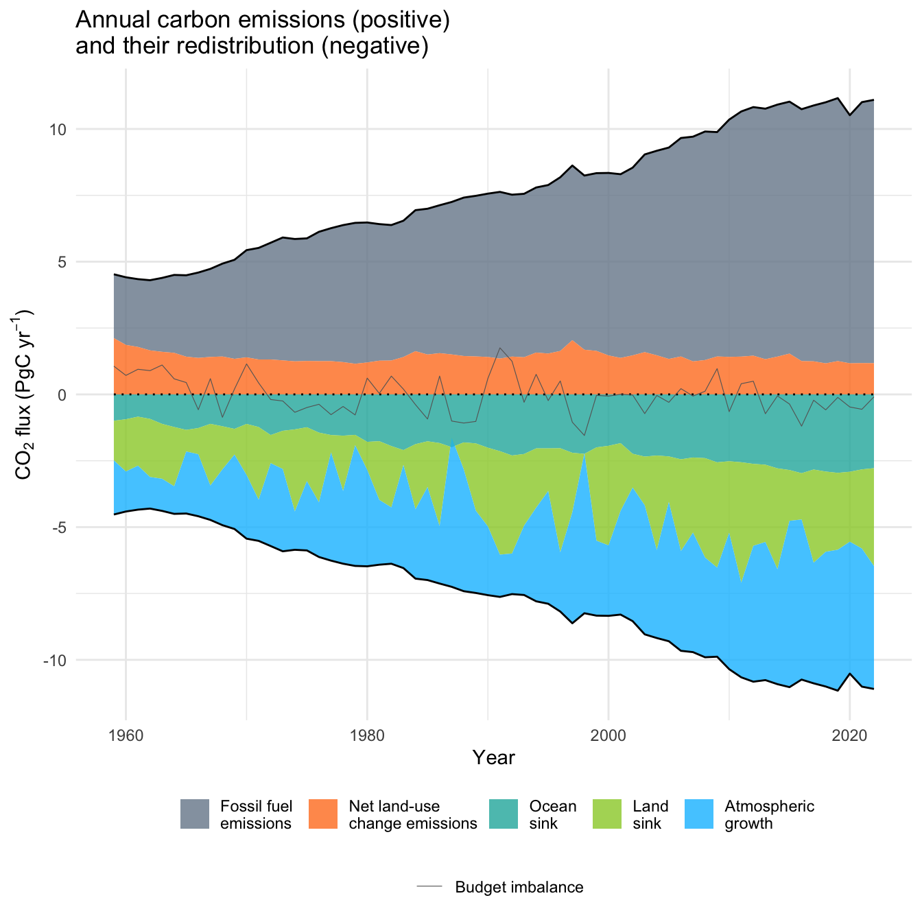

Figure 3.4: Annual carbon emissions (positive) and their redistribution between the ocean, land, and atmosphere (negative). The black line in the positive domain represents total emissions and is mirrored by the black line in the negative domain which represents the total of the land sink, ocean sink, and atmospheric growth. Design and data are based on the Global Carbon Budget. In contrast to Friedlingstein et al. (2023), the land sink is defined here as the carbon budget residual. The budget imbalance term - the difference between S_land calculated as the budget residual vs. bottom-up using land C cycle models - is shown by the separate fine grey line.

3.4 Understanding the land C sink

3.4.1 Processes

As challenging as it was to locate the “missing C sink” in the terrestrial biosphere in the 1990s (see above), it remains a great challenge to locate the C sink within the terrestrial biosphere and attribute it to processes. Three processes are considered to be particularly influential for the terrestrial C balance, and they each affect ecosystems’ C balances in different regions across the globe - land use change, the relief of temperature limitations on photosynthesis and growth, and the CO₂ fertilization effect.

The land C balance from land use change is the net of a flux to the atmosphere due to deforestation and a flux from the atmosphere to the land biosphere due to regrowth after deforestation. Land use change trends are very different across regions globally. While large C losses due to land use change are currently occurring in the tropics, northern extra-tropical regions generally gain C as forests are recovering from more intense wood harvesting in the past - prior the the mid-20th century. Chapter 10 delves deeper into the role of land use change on the carbon cycle and climate. The net C flux from land use change is accounted for in the global carbon budget by the term $E_{\mathrm{LUC}}$ (Equation 3.6) and should reflect also effects by C accumulation in recovering forests. However, past land use changes are uncertain and the impact of pre-1950 wood harvesting in temperate regions may be underestimated by models that supply estimates for $E_{\mathrm{LUC}}$. $S_{\mathrm{land}}$, when defined as the budget residual, may thus be driven by the C sink in recovering forests. A recent estimate suggests that about a quarter of the land sink, or 1.3 PgC yr^-1, is due to recovery from past forest disturbances (fire, wind, and wood harvesting) (Pugh et al. 2019).

Warming trends due to anthropogenic climate change are relieving temperature limitations on photosynthesis and tree growth, enabling an extension of the growing season (Ruehr et al. 2023), and an expansion of forest areas and vegetation greenness in high northern latitudes - as sensed from space (T. F. Keenan and Riley 2018). The associated land C sink, as the one driven by forest recovery from past land use change, is located in the northern extra-tropics.

Rising atmospheric CO₂ stimulates leaf-level photosynthetic rates. The additional C assimilated likely drives increases in ecosystem C storage. However, a multitude of processes and ecosystem feedbacks are involved and affect the link between the leaf-level CO₂-fertilization of photosynthesis and ecosystem-level C storage (nutrient limitation, tree longevity reduction due to accelerated growth, soil organic C loss due to plant-soil interactions). Free-Air-CO₂-Experiments, where plots of outdoor growing vegetation are exposed to elevated CO₂ during multiple years indicate a stimulation of photosynthesis and growth, but evidence for gains in biomass and soil C stocks is mixed. Yet, C gains in mature forest growth, biomass, and ecosystem C stocks are documented and, particularly in the tropics, CO₂-fertilization appears to be the main driver of this trend. This is consistent with Dynamic Global Vegetation Models that attribute about 60-85% of the total land sink to CO₂-fertilization (Schimel, Stephens, and Fisher 2015; Trevor F. Keenan et al. 2016). Published review studies (Ruehr et al. 2023; Walker et al. 2021) provide a more detailed account of the complex role of CO₂-fertilization in driving the land C sink.

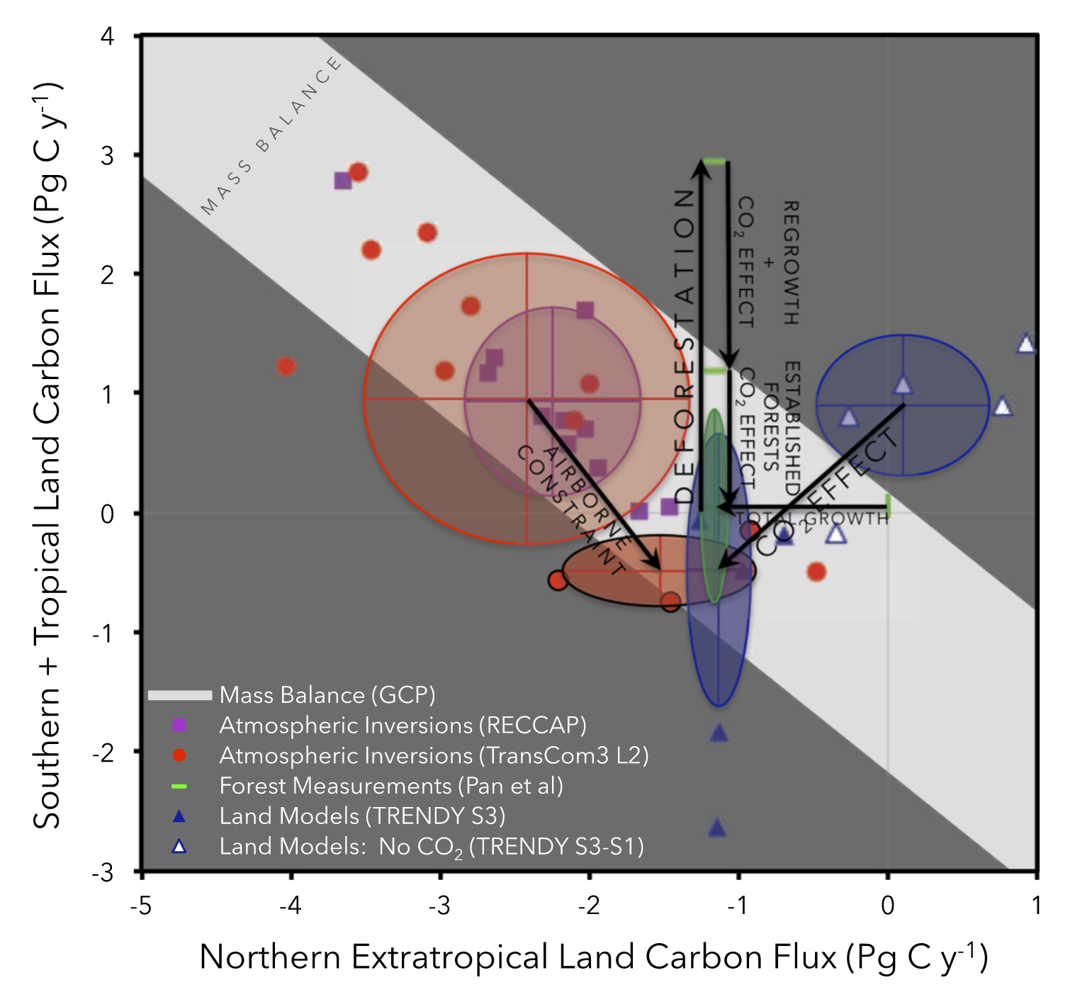
Theory suggests that the CO₂ effect on photosynthesis should be higher under warm than under cold temperatures. Therefore, a CO₂-driven land sink should be strongest in the tropics. As mentioned above, a C sink that is driven predominantly by either growing season extensions and cold limitation reliefs or by recovery from past land use change would be located mainly in the northern extra-tropics. How to discriminate between these drivers and their associated C sink regions? Once more, atmospheric CO₂ measurements provide a constraint. While the total terrestrial C sink is relatively well-constrained through the global carbon budget, contributions from the tropics (and southern hemisphere) vs. the northern extra-tropics requires an additional constraint. Atmospheric CO₂ measurements, in combination with known CO₂ sources and their location and with atmospheric transport fields (atmospheric inversions) enable a split of the global land C sink into contribution from the two regions, while their sum is constrained by the global carbon budget. This approach is visualized in Figure 3.5. The combination of the two constraints indicates that model simulations where the CO₂-fertilization effect was “turned off” tend to be outside the range of plausible combinations of tropical and northern-extratropical land C sinks. This indicates the importance of a strong CO₂-fertilization-driven C sink in the tropics. Hence, the hypothesis that the land C sink is driven exclusively by forest recovery from past land use and the extension of the growing season in cold-limited regions of the northern extra-tropics is not compatible with the C budget and the inter-hemispheric split of land C uptake inferred from atmospheric inversions.

Figure 3.5: The anti-correlation of the northern extra-tropical and the tropical-plus-southern land C sink. Atmospheric inversions from different sources (red and purple points and squares) indicate an anti-correlation of the regional sinks, constrained by the C mass balance from the global carbon budget: The sum of regional land C sinks must equal the total terrestrial C sink from the global carbon budget. Several Dynamic Global Vegetation Models (DGVMs) without the CO₂-fertilisation effect (white triangles) lie outside the range constrained by the global C mass balance, while DGVMs with the CO₂-fertilisation effect considered are better compatible with the budget. Figure from Schimel, Stephens, and Fisher (2015).

The processes for understanding the oceanic C sink will be introduced in Chapter 13.

3.4.2 Interannual variability

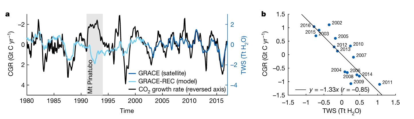
As highlighted above, pointing to Figure 3.4, the magnitude of the land C sink varies strongly between years. Semi-arid regions, where dry conditions during a substantial part of the year limit photosynthesis and where drought-related disturbances strongly influence ecosystem C balances, are contributing most strongly to the signal apparent from the global C budget (Ahlström et al. 2015). Semi-arid regions largely align with temperate and tropical grasslands, savannahs, and shrubland biomes (Figure 2.2). Years with a small land sink and a high atmospheric CO₂ growth rate are dry years, associated with low global-scale terrestrial water storage (Humphrey et al. 2018), and are associated with warm temperature anomalies in the tropics (Cox et al. 2013). This indicates two important points. First, C storage in the terrestrial biosphere is highly susceptible to climate variations. Second, water availability has a strong control on the terrestrial carbon cycle. We will learn more about how the water and the carbon cycles are coupled in Chapter 7 and how the influence of water availability on vegetation varies across the globe in Chapter 8.

Figure 3.6: Interannual variability of the atmospheric CO₂ growth rate (CGR) and terrestrial water storage (TWS). (a) Monthly de-seasonalized and de-trended CGR, TWS from gravimetric satellite observations (GRACE mission) and TWS from a statistical model that reconstructs the TWS based on climate data (GRACE-REC). The vertical axis is inverted for CGR so that positive (downwards) CGR anomalies indicate a weaker land carbon sink. A 6-month moving average was applied to GRACE data for readability. (b) Yearly CGR versus GRACE TWS anomalies. Figure and caption text from Humphrey et al. (2018).

CO₂ trajectories and the land C cycle response

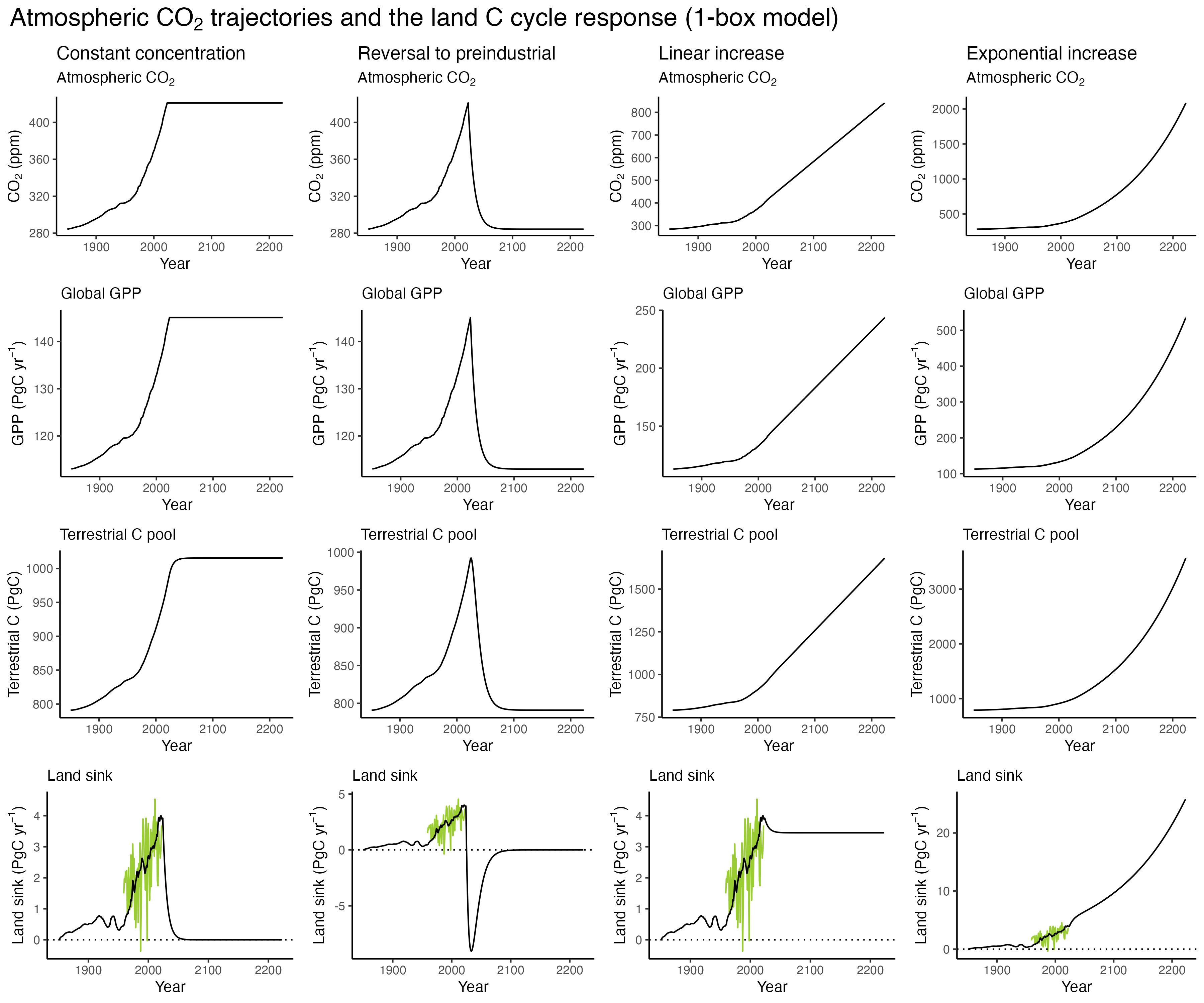
Equation 3.2 describes the dynamics of land C storage based on a 1-box model. Let’s apply this model for understanding the link between changes in $I$ and the land C balance ($\mathrm{d}C/\mathrm{d}t$). We explore different future trajectories of atmospheric CO₂, branching off from its observed history, and simulate the resulting total terrestrial photosynthetic CO₂ uptake (also referred to as the gross primary productivity, see also Chapter 4), the terrestrial C pool, and the land sink (i.e., the temporal change in the terrestrial C pool).

We make the (strong) assumption that the land C balance dynamics are exclusively driven by the CO₂-fertilization effect on photosynthetic C uptake, represented by $I$, while the turnover rate ($\tau$) remains constant. The CO₂-fertilization effect on a variable $x$ is commonly measured as the sensitivity factor $\beta$: $$\begin{array}{}\text{(3.8)}& \beta =\frac{\ln (x/x_0)}{\ln (c_a/c_{a,0})}\end{array}$$ Here, $c_a$ is the atmospheric CO₂ concentration (ambient CO₂). For ratios of $x/x_0$ and $c_a/c_{a,0}$ approaching 1, Equation 3.8 is equivalent to the ratio of the relative change in $x$ over the relative change in CO₂. $$\begin{array}{}\text{(3.9)}& \beta \approx \frac{\mathrm{\Delta }x/x}{\mathrm{\Delta }{c}_a/c_a},\end{array}$$ where $\mathrm{\Delta }x=x-x_0$. The sensitivity of the total terrestrial photosynthetic CO₂ uptake to atmospheric CO₂ has been estimated by T. F. Keenan et al. (2023) as $\beta =0.59\pm 0.16$. With this, we can model $I$ as a function of $c_a$ using Equation 3.9.

The 1-box model can be implemented numerically by discretization in time (i.e., considering time steps $\mathrm{\Delta }t$). To simulate the terrestrial C pool over time ($C(t)$), Equation 3.2 can thus be written as $$C(t+\mathrm{\Delta }t)=C(t)+I(t)-{\tau }^{-1}C(t)$$

We further assume that $C(t)$ was at steady-state in year 1850 - the first year of the CO₂ time series used here. $\tau$ could be estimated by using values of terrestrial C pools (sum of vegetation C and soil C) and the gross photosynthesis flux from Figure 3.1 ($\tau =(450\mathrm{GtC}+1700\mathrm{GtC})/113{\mathrm{GtC}\mathrm{yr}}^{-1}=19.0\mathrm{yr}$). However, the resulting land C sink would be strongly overestimated when compared to the residual sink $S_{\mathrm{land}}$ from the Global Carbon Budget. When choosing $\tau =9\mathrm{yr}$, a better fit between the 1-box model-derived land sink and the observed land sink emerges. This could indicate that CO₂-fertilization drives additional C storage that is more short lived than on average in vegetation and soil biomass. It probably also indicates that not all of the C assimilated by photosynthesis stays in the system for more than a few minutes to weeks. A substantial fraction of that C is respired by plants (autotrophic respiration, see also Chapter 4) before it is synthesized into longer-lived plant tissue biomass. The resulting evolution(s) of the land C cycle are illustrated in Figure 3.7.

Figure 3.7: Evolution of the land C cycle in response to alternative (schematic) trajectories of future CO₂. The green line in panels of the bottom row indicates the observed land sink, derived as the residual of the Global Carbon Budget.

Exercise

6. Express $I$ as a function of $c_a$, using the definition of $\beta$ from Equation 3.9, and using $c_{a,0}$ and $I_0$.
7. Calculate $I(c_a)$ for $c_a=400$ ppm and $I_0$ as the pre-industrial value of total terrestrial gross photosynthesis from Figure 3.1 and using the value of $\beta$ (mean) from T. F. Keenan et al. (2023).
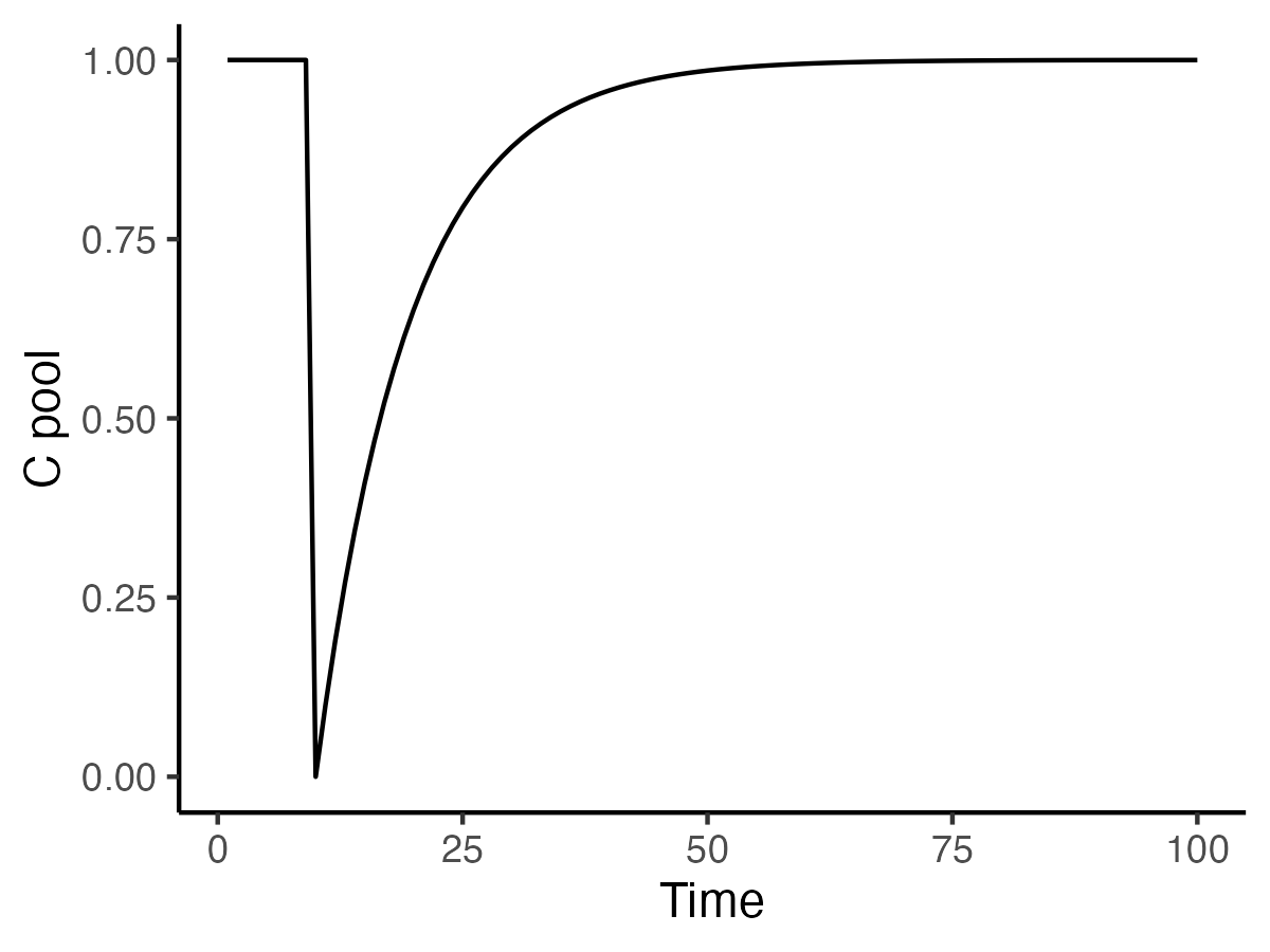
8. It is important to note that the land C sink trajectories are strongly dependent on whether the dominating process driving it is CO₂ fertilization or forest recovery from past disturbance (or other drivers). The temporal course of ecosystem C pools after a disturbance is schematically illustrated in Figure 3.8. Sketch the resulting land C sink for the different CO₂ trajectories of Figure 3.7 if the sink was exclusively driven by forest recovery.

Figure 3.8: Schematic illustration of the recovery of the ecosystem C pool (relative magnitude) after a disturbance in time step 10.

Ahlström, Anders, Michael R. Raupach, Guy Schurgers, Benjamin Smith, Almut Arneth, Martin Jung, Markus Reichstein, et al. 2015. “The Dominant Role of Semi-Arid Ecosystems in the Trend and Variability of the Land CO2 Sink.” Science 348 (6237): 895–99. https://doi.org/10.1126/science.aaa1668.

Ballantyne, A. P., C. B. Alden, J. B. Miller, P. P. Tans, and J. W. C. White. 2012. “Increase in Observed Net Carbon Dioxide Uptake by Land and Oceans During the Past 50 Years.” Nature 488 (7409): 70–72. https://doi.org/10.1038/nature11299.

Canadell, J. G., P. M. S. Monteiro, M. H. Costa, L. Cotrim da Cunha, P. M. Cox, A. V. Eliseev, S. Henson, et al. 2021. “Global Carbon and Other Biogeochemical Cycles and Feedbacks.” Book Section. In Climate Change 2021: The Physical Science Basis. Contribution of Working Group i to the Sixth Assessment Report of the Intergovernmental Panel on Climate Change, edited by V. Masson-Delmotte, P. Zhai, A. Pirani, S. L. Connors, C. Péan, S. Berger, N. Caud, et al., 673–816. Cambridge, United Kingdom; New York, NY, USA: Cambridge University Press. https://doi.org/10.1017/9781009157896.007.

Cox, Peter M., David Pearson, Ben B. Booth, Pierre Friedlingstein, Chris Huntingford, Chris D. Jones, and Catherine M. Luke. 2013. “Sensitivity of Tropical Carbon to Climate Change Constrained by Carbon Dioxide Variability.” Nature 494 (7437): 341–44. https://doi.org/10.1038/nature11882.

Elsig, Joachim, Jochen Schmitt, Daiana Leuenberger, Robert Schneider, Marc Eyer, Markus Leuenberger, Fortunat Joos, Hubertus Fischer, and Thomas F Stocker. 2009. “Stable Isotope Constraints on Holocene Carbon Cycle Changes from an Antarctic Ice Core.” Nature 461 (7263): 507–10. https://doi.org/10.1038/nature08393.

Falkowski, P., R. J. Scholes, E. Boyle, J. Canadell, D. Canfield, J. Elser, N. Gruber, et al. 2000. “The Global Carbon Cycle: A Test of Our Knowledge of Earth as a System.” Science 290 (5490): 291–96. https://doi.org/10.1126/science.290.5490.291.

Friedlingstein, P., M. O’Sullivan, M. W. Jones, R. M. Andrew, D. C. E. Bakker, J. Hauck, P. Landschützer, et al. 2023. “Global Carbon Budget 2023.” Earth System Science Data 15 (12): 5301–69. https://doi.org/10.5194/essd-15-5301-2023.

Humphrey, Vincent, Jakob Zscheischler, Philippe Ciais, Lukas Gudmundsson, Stephen Sitch, and Sonia I. Seneviratne. 2018. “Sensitivity of Atmospheric CO2 Growth Rate to Observed Changes in Terrestrial Water Storage.” Nature 560 (7720): 628–31. https://doi.org/10.1038/s41586-018-0424-4.

Joos, Fortunat, and Michele Bruno. 1998. “Long-Term Variability of the Terrestrial and Oceanic Carbon Sinks and the Budgets of the Carbon Isotopes 13C and 14C.” Global Biogeochemical Cycles 12 (2): 277–95. https://doi.org/10.1029/98GB00746.

Keeling, Ralph F., Stephen C. Piper, and Martin Heimann. 1996. “Global and Hemispheric CO2 Sinks Deduced from Changes in Atmospheric O2 Concentration.” Nature 381 (6579): 218–21. https://doi.org/10.1038/381218a0.

Keenan, T. F., X. Luo, B. D. Stocker, M. G. De Kauwe, B. E. Medlyn, I. C. Prentice, N. G. Smith, et al. 2023. “A Constraint on Historic Growth in Global Photosynthesis Due to Rising CO2.” Nature Climate Change, November, 1–6. https://doi.org/10.1038/s41558-023-01867-2.

Keenan, T. F., and W. J. Riley. 2018. “Greening of the Land Surface in the World’s Cold Regions Consistent with Recent Warming.” Nature Climate Change 8 (9): 825–28. https://doi.org/10.1038/s41558-018-0258-y.

Keenan, Trevor F., I. Colin Prentice, Josep G. Canadell, Christopher A. Williams, Han Wang, Michael Raupach, and G. James Collatz. 2016. “Recent Pause in the Growth Rate of Atmospheric CO2 Due to Enhanced Terrestrial Carbon Uptake.” Nature Communications 7 (1): 13428. https://doi.org/10.1038/ncomms13428.

Li, Changyu, Jianping Huang, Lei Ding, Yu Ren, Linli An, Xiaoyue Liu, and Jiping Huang. 2022. “The Variability of Air-Sea O2 Flux in CMIP6: Implications for Estimating Terrestrial and Oceanic Carbon Sinks.” Advances in Atmospheric Sciences 39 (8): 1271–84. https://doi.org/10.1007/s00376-021-1273-x.

Pugh, Thomas A. M., Mats Lindeskog, Benjamin Smith, Benjamin Poulter, Almut Arneth, Vanessa Haverd, and Leonardo Calle. 2019. “Role of Forest Regrowth in Global Carbon Sink Dynamics.” Proceedings of the National Academy of Sciences 116 (10): 4382–87. https://doi.org/10.1073/pnas.1810512116.

Ruehr, Sophie, Trevor F. Keenan, Christopher Williams, Yu Zhou, Xinchen Lu, Ana Bastos, Josep G. Canadell, Iain Colin Prentice, Stephen Sitch, and César Terrer. 2023. “Evidence and Attribution of the Enhanced Land Carbon Sink.” Nature Reviews Earth & Environment 4 (8): 518–34. https://doi.org/10.1038/s43017-023-00456-3.

Schimel, David, Britton B. Stephens, and Joshua B. Fisher. 2015. “Effect of Increasing CO2 on the Terrestrial Carbon Cycle.” Proceedings of the National Academy of Sciences 112 (2): 436–41. https://doi.org/10.1073/pnas.1407302112.

Shanahan, Timothy M., Nicholas P. McKay, Konrad A. Hughen, Jonathan T. Overpeck, Bette Otto-Bliesner, Clifford W. Heil, John King, Christopher A. Scholz, and John Peck. 2015. “The Time-Transgressive Termination of the African Humid Period.” Nature Geoscience 8 (2): 140–44. https://doi.org/10.1038/ngeo2329.

Sierra, Carlos A., Markus Müller, Holger Metzler, Stefano Manzoni, and Susan E. Trumbore. 2017. “The Muddle of Ages, Turnover, Transit, and Residence Times in the Carbon Cycle.” Global Change Biology 23 (5): 1763–73. https://doi.org/10.1111/gcb.13556.

Walker, Anthony P., Martin G. De Kauwe, Ana Bastos, Soumaya Belmecheri, Katerina Georgiou, Ralph F. Keeling, Sean M. McMahon, et al. 2021. “Integrating the Evidence for a Terrestrial Carbon Sink Caused by Increasing Atmospheric CO ${}_{\text{2}}$.” New Phytologist 229 (5): 2413–45. https://doi.org/10.1111/nph.16866.