Forcing
BGC simulations
For Landcover6K-BGC simulations with constant climate and CO2 (bgc_luXX_clim0, see Protocols), only the land use forcing is specified explicitly. Climate and CO2, and other forcings depending on the model, are to be held constant at pre-industrial values. We recommend modelling groups to follow established protocols for running models with constant preindustrial conditions, as commonly applied in other model intercomparison projects (e.g., piControl in CMIP6). Required information to fully specify the LULC forcing for Landcover6K-BGC simulations are described below. LULC forcing files are provided at three spatial resolutions (see tabs: 2.5 \(\times\) 3.75\(^{\circ}\), 1\(^{\circ}\) and 0.5\(^{\circ}\)), along with corresponding land mask files. An example for how the LULC forcing was specified in Stocker et al. (2017) is given in the tab ‘Example’. Information on Agricultural system is required for the model implementation to specify gross land use transitions (shifting cultivation, fallow rotations, see Implementation, and to specify additional parameters describing the land use system and how it is “translated” for model simultations
In the simulation with varying climate and CO2 (bgc_lu00_clim1, see Protocols), LULC is zero. Other temporally varying forcings to be applied for this simulation, are described in section ‘Other forcings’.
LULC forcings overview
Example
| Variable | File name | Variable name | Reference | Remarks |
|---|---|---|---|---|
| Land mask | landmask_pelt04_rs_lpjgr.cdf | LAND | Peltier (2004) | Land: LAND = 2. Ice-covered: LAND = 0. Use last time slice for all time step (constant present-day mask). |
| Cropland area fraction | landuse_hyde32_baseline_pastcorr_lpjgr.nc | crop | Klein Goldewijk (2016) | |
| Pasture area fraction | landuse_hyde32_baseline_pastcorr_lpjgr.nc | past | Klein Goldewijk (2016) | Naturally open vegetation cover, simulated by LPX under preindustrial conditions, is subtracted from the pasture area fraction given by HYDE 3.2. |
| Harvested area fraction | harvest_hurtt_byarea_v2_lpjgr_backby_hyde32_baseline.nc | aharv | Hurtt et al. (2006) | Defines the (forest) area that is cleared per year. Used Hurtt et al. (2006) data and back-projected by continent in proportion to cropland area |
| Agricultural system | perm_lpjgr_holoLU2.nc | PERM | Butler (1980); Hurtt et al. (2006); Stocker et al. (2017) | Here a boolean. Defines whether 100% of cropland area in this gridcell is to be treated as shifting cultivation or not. |
2.5 \(\times\) 3.75\(^{\circ}\)
| Variable | File name | Variable name | Reference | Remarks |
|---|---|---|---|---|
| Land mask | landmask_pelt04_rs_lpjgr.cdf | LAND | Peltier (2004) | Land: LAND = 2. Ice-covered: LAND = 0. Use last time slice for all time step (constant present-day mask). |
| Cropland area fraction | landuse_hyde32_baseline_pastcorr_lpjgr.nc | crop | Klein Goldewijk (2016) | |
| Pasture area fraction | landuse_hyde32_baseline_pastcorr_lpjgr.nc | past | Klein Goldewijk (2016) | Naturally open vegetation cover, simulated by LPX under preindustrial conditions, is subtracted from the pasture area fraction given by HYDE 3.2. |
| Harvested area fraction | harvest_hurtt_byarea_v2_lpjgr_backby_hyde32_baseline.nc | aharv | Hurtt et al. (2006) | Defines the (forest) area that is cleared per year. Used Hurtt et al. (2006) data and back-projected by continent in proportion to cropland area |
| Agricultural system | perm_lpjgr_holoLU2.nc | PERM | Butler (1980); Hurtt et al. (2006); Stocker et al. (2017) | Boolean. Defines whether 100% of cropland area in this gridcell is to be treated as shifting cultivation or not. |
1\(^{\circ}\)
| Variable | File name | Variable name | Reference | Remarks |
|---|---|---|---|---|
| Land mask | ||||
| Cropland area fraction | ||||
| Pasture area fraction | ||||
| Harvested area fraction | ||||
| Agricultural system |
0.5\(^{\circ}\)
| Variable | File name | Variable name | Reference | Remarks |
|---|---|---|---|---|
| Land mask | ||||
| Cropland area fraction | ||||
| Pasture area fraction | ||||
| Harvested area fraction | ||||
| Agricultural system |
LULC forcings description
Cropland area
Gridcell area fraction. Specifies the area used for crop cultivation at a given point in time. This excludes fallow fields.
Pasture area
Gridcell area fraction. This defines the extent of land that is regularly grazed. Note that naturally open vegetation is assumed to be used before any forest is cleared to satisfy expanding pasture areas. If the balance between open land and closed forests is dynamically simulated by the model, a reduced pasture extent that fully comes at the expense of the simulated potential natural vegetation has to be derived offline beforehand. On land used for pasture, aboveground biomass is to be removed periodically and should not be added to litter pools (but respective C to be respired directly as CO2). No land turnover is simulated for pasture. In areas of mobile or transhumant pastoralism, the annual aboveground biomass removal fraction is to be set to a lower value.
Urban area
Gridcell area fraction. Due to the relatively small area covered by urban, built-up lands during the preindustrial period, we neglect this land use class for BGC simulations.
Harvested area
Gridcell area fraction Defines the (forest) area that is cleared per year to satisfy demand for wood (construction, smeltering).
Agricultural system
Categorical. This is to define the spatial distribution of Level-2 land use classes at different points in time (planned 6 and 2 ka BP) after Morrison et al. (2018) (see Figure below). The classification is used to define a set of land use parameters that characterise typical practices for each category (agricultural system) and that are directly translatable into model implementations for Landcover6K-BGC (and ESM?) simulations. Land use parameters required by models are:
- Fallow duration (\(\tau_f\))
- Duration of cultivation between fallow periods (\(\tau_c\))
- Whether or not croplands are irrigated (alleviating all soil moisture limitation in BGC models, and setting annual precipitation on respective land to potential evapotranspiration minus precipitation (PET-P) in ESMs.)
- Whether or not litter inputs are reduced (crop harvesting and off-site decomposition of residues, absence of mulching) and/or soil organic matter decomposition is accelerated by cultivation (e.g., tillage). This information is important for simulating soil C stocks and their responses to land use change.
A lookup table can then be used to associate the Level-2 classification with required land use parameters for its implementation in models:
| Level 2 class | \(\tau_f\) (yr) | \(\tau_c\) (yr) | Irrigated croplands | Reduced soil C |
|---|---|---|---|---|
| Tropical intensive agroforestry | 0 | inf. | FALSE |
??? |
| Swidden/shifting cultivation | 15 | 3.0 | FALSE |
TRUE |
| Industrial monocrop/plantation | 0 | inf. | FALSE |
TRUE |
| Flooded field farming | 0 | inf. | FALSE |
TRUE |
| Non-irr. annual cropping w/ animals | 1 | 2.0 | FALSE |
TRUE |
| Non-irr. annual cropping w/o animals | 1 | 2.0 | FALSE |
TRUE |
| Irr. annual cropping w/ animals | 0 | inf. | TRUE |
TRUE |
| Irr. annual cropping w/o animals | 0 | inf. | TRUE |
TRUE |
| Pastoralism, sedentary | NA | NA | FALSE |
TRUE |
| Pastoralism, mobile/transhumant | NA | NA | FALSE |
TRUE |
Other inormation from the Level-1/Level-2 land use classification are not relevant as model forcing. More information on how to use parameters to define land use transitions is given in Implementation.
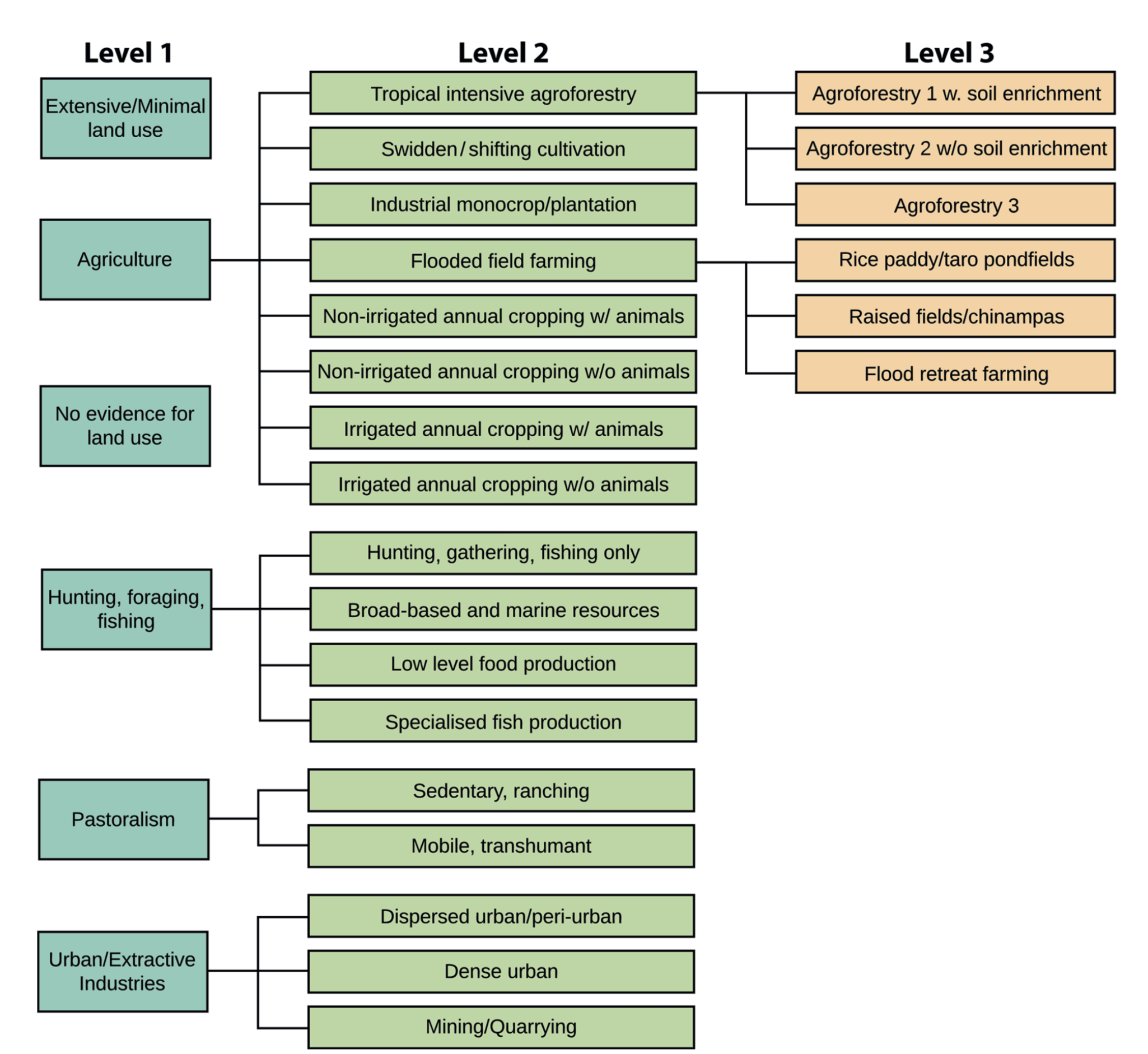
The LandCover6k land-use classification after Morrison et al., 2018.
To consider:
The Level-2 land use classification maps are given at a high spatial resolution (10 km). Model forcing datasets are required at a much lower spatial resolution. Aggregating from the original dataset to the model forcing dataset may either be done using the most frequent class within each coarse-resolution gridcell, or the model forcing could be defined as the fractional shares of each Level-2 class within each coarse-resolution gridcell. This would lead to 10 variables. E.g., specifying \(f_1\) the share of Tropical intensife agroforestry, \(f_2\) specifying the share of Swidden/shifting cultivation, etc. as a fraction of total agricultural (or cropland) area. And \(\sum_i f_i =1\).
Other forcings
Orbital parameters
We recommend the application of transiently varying orbital parameters based on Berger et al. (1978). Fortran code for calculating eccentricity, obliquity, and the longitude of perihelion can be accessed here.
CO2
A time series for globally uniform mean atmospheric CO2 concentration per year, based on data from Monnin et al. (2001), Monnin et al. (2004), and Siegenthaler et al. (2005), can be accessed here. The data was prepared by F. Joos (pers. comm.).
Climate
Climate forcing data will be provided from an existing transient climate simulation made with the ECHAM model (Fischer and Jungclaus, 2011). Files cover years 6 ka BP to present-day transiently (i.e., in discrete time slices, with linear interpolation recommended for year in between), at the same spatial resolution as the landmask and LULC forcings.